Micro CT · Application note
X-Ray Sources for Micro CT and Industrial CT Systems
- Published 13 October 2026
- 22 min read
- Curpow application engineering
Short answer
Set the focal spot equal to the voxel size, at the power the scan actually runs at. Spot diameter grows about 1 µm per watt, so ask for a spot against power curve, not a single minimum. The CX40 reaches 4.5 µm, the CX20 carries 25 W, and the CX30 reaches 130 kV.
On this page
- What manufacturers use micro CT to inspect
- Micro CT, nanofocus CT and conventional CT compared
- In-line CT and lab CT, where each belongs
- What voxel size a micro CT system needs, and how the source sets it
- How focal spot size changes with tube power
- How to choose tube voltage for micro CT
- Spot position stability over a scan that runs for hours
- Focus to object distance and the magnification your part leaves you
- Choosing between the CX20, CX30, and CX40 for a micro CT system
- Lead time and second sourcing
- How to specify an X-ray source for your CT system
- What this means for your source selection
- Sources
A micro CT scanner takes hundreds of X-ray pictures of a part. The part sits on a turntable that rotates a fraction of a degree between pictures, so each picture looks through the part from a slightly different angle. A computer then stacks those pictures into a model the operator can slice open on screen, without ever cutting the part. A scanner builder designs every machine of this kind around one bought-in component, the X-ray source, and the source sets the limit on how small a detail the finished scanner can show.
National metrology institutes and failure analysis labs have already published what a CT system needs from its source: the voltage that gets through the part, the focal spot small enough for the detail they wanted to see, how far the spot may drift before a long scan reconstructs badly, and how close the part can sit to the spot. We took those published numbers and checked the CX20, CX30, and CX40 against every one of them. So you can read the requirements and our specifications in the same place.
This page works through the source specifications in the order a CT builder decides them. Where the voxel size comes from. Focal spot size at the power a scan actually runs. Tube voltage against the material in the part. Spot position stability across a scan that lasts hours. And the focus to object distance that decides how much geometric magnification your part leaves you. It closes with the CX20, CX30, and CX40 side by side, and how to write the specification yourself.
Key takeaways
- A micro CT scanner resolves only what its source resolves. The focal spot casts a blur through the part, and that blur does not shrink when the reconstruction samples more finely. So the source sets the ceiling for the whole machine, whatever the detector and the algorithm do afterwards.
- Pick the voxel from the smallest feature your customer must see, then buy a spot to match it. Published practice sets tube power at the point where spot diameter is about the same as voxel size. A smaller spot costs exposure time you did not need to spend. A larger spot wastes the sampling you paid the detector for.
- Focal spot diameter grows by roughly 1 µm for every watt you add. About 99 percent of what an X-ray tube consumes leaves as heat, and the target survives only so much heat per unit area. A data sheet quoting a minimum focal spot and a maximum power quotes two numbers that never occur together.
- Voltage follows the part, not the application. Published CT scans ran 80 kV on a few millimetres of ruby, 145 kV on a 30 mm aluminium printed part, and above 100 kV on copper and solder inside packages. At the top of that range the spot blooms, which costs resolution.
- Over a scan lasting hours, spot position stability decides whether the reconstruction is usable at all. One national metrology institute measured about 10 µm of uncompensated tube expansion on a scan reconstructed at a 2.1 µm voxel, then nearly halved its measurement error by correcting for it. Warm the source up before the scan starts.
- The CX20, CX30, and CX40 each take a different corner of CT work. The CX40 holds the smallest focal spot in the range at 4.5 µm and sits 6.0 mm from the part. The CX20 carries the most flux at 25 W and reaches 110 kV. The CX30 reaches 130 kV, publishes its full focal spot against tube power curve, and lists a highly stable spot position for CT and 3D.
What manufacturers use micro CT to inspect
A CT system builder sells the scan, not the scanner. So the feature sizes your customers need to see fix your source specification. Published micro CT work covers five kinds of inspection:
- Porosity and voids in printed metal parts. One study scanned an aluminium flexure hinge of 30 mm by 12 mm by 5 mm against a reference pin. That pin carried calibrated holes of 30, 50, 90, and 120 µm. At an 8.5 µm voxel the 30 µm holes were the difficult case, so the authors called for the smallest voxel the geometry allows.
- Voids and cracks in solder joints and copper vias. A review of CT in semiconductor packaging by Intel and Lawrence Livermore reports two limits on 2D radiography. A single radiograph cannot capture voids smaller than 5 µm in diameter, even in the best case. A single radiograph also cannot separate two voids that overlap in the beam path. Substrate copper via defects usually run smaller than 5 µm.
- Column and ball position in area array assemblies. A NASA Jet Propulsion Laboratory study put column grid array assemblies and four-high stacked packages through CT after thermal cycling, and used the reconstruction to measure column tilt.
- Traceable dimensional measurement on small precision parts. The Swiss federal metrology institute scanned a standard of 22 ruby spheres, each 0.3 mm across and 3.6 mm across the whole set. The institute then compared 231 sphere centre to centre distances against a tactile measurement calibrated to 0.08 µm.
- Internal geometry no probe can reach. The National Physical Laboratory reported an international audit of industrial CT systems, in which participants measured inner and outer cylinder diameters, sphere centre distances, and the smallest cylindrical micro structure on reference artefacts. Distances came out more accurate than diameters, and diameters more accurate than form error.
| Part scanned | Tube voltage | Tube power | Voxel or resolution | Projections and scan time | What that asks of the source |
|---|---|---|---|---|---|
| 22 ruby spheres, 0.3 mm each, 3.6 mm overall | 80 kV | 5 W | 2.1 µm | 3,000 projections, 5 hours | A spot of a few µm at 5 W, held still for five hours |
| Aluminium printed flexure, 30 mm by 12 mm by 5 mm | 145 kV | 41 µA, about 6 W | 8.5 µm | 1,650 projections | High kV at low power, so the spot stays near the voxel |
| Semiconductor package, 1 to 2 mm² field of view | above 100 kV | not stated | micrometre level | several hours per field of view | Flux at a small spot, because exposure time is the constraint |
| System in package, 16 mm by 16 mm | 4 to 100 kV, synchrotron beam | not applicable | 4.5 to 8.7 µm | 3 to 20 minutes | The benchmark a lab source has to answer to |
Ruby sphere standard from Bircher et al. 2020; printed flexure from Chahid et al. 2024; semiconductor package and system in package from Li et al. 2014; reference artefact audit from Sun et al. 2012. Full references at the foot of the page.
Micro CT, nanofocus CT and conventional CT compared
Focal spot size separates the three classes, and the National Physical Laboratory draws the lines by focal spot size alone.
| Class | Focal spot | Smallest detail it can resolve | What it suits |
|---|---|---|---|
| Conventional CT | larger than 1 mm | Blur of roughly a millimetre, whatever the magnification | Large objects, where the smallest detail runs to millimetres |
| Microfocus CT, or micro CT | 1 µm to 1000 µm | Micrometre-scale detail, once the part sits close to the spot | Industrial CT scanning, 3D inspection, and dimensional metrology |
| Nanofocus CT | smaller than 1 µm | Sub-micrometre detail | Research and failure analysis, at low power and long scan times |
Focal spot bands from Sun et al. 2012.
Industrial CT also works differently from medical CT, and that difference costs a CT builder more than the focal spot bands do. Industrial CT rotates the part in front of a fixed source and detector. So the part has to fit between the source and the detector, and the part has to clear the source housing every time it comes round. A large part therefore cannot get close to the focal spot, and how close a part gets to the focal spot decides the magnification your machine can reach.
In-line CT and lab CT, where each belongs
Lab CT buys resolution with time. A dimensional CT scan of a 3.6 mm sphere standard at a 2.1 µm voxel took 3,000 projections and five hours. The Intel and Lawrence Livermore review puts the general figure at several hours of acquisition per 1 to 2 mm² region of interest, against packages that run 100 to 3,600 mm². Nobody puts a several-hour scan on a production line.
In-line CT buys time by giving up projections and spot size. A survey of high-speed laboratory CT found the fastest commercial scan at 9.4 seconds. The same survey found that most operators do not meet the Nyquist sampling criterion, which asks for the detector window size multiplied by π/2 projections, and that the average across the studies surveyed was 60 percent of that count. Two by two detector binning brightens the image four times, so the exposure per projection drops proportionally.
So an in-line scan and a lab scan ask opposite things of the same source. The in-line scan wants flux, because exposure time per projection is the whole budget. The lab scan wants the smallest stable spot, because a lab scan can afford to wait. The CX20 carries the most power in the Curpow range at 25 W, and its data sheet names micro-CT alongside high flux and spot location stability. The CX30 data sheet lists a high reliability design for in-line applications and a highly stable spot position for CT and 3D. An automated inspection cell needs both claims.
Intel’s own stated requirement for a next-generation laboratory CT source names three things:
- Enough magnification on a full-size sample that nobody has to trim it down to reach micrometre resolution.
- High brightness across an energy range of 40 to 150 kV, so the beam handles copper and solder while still imaging the dielectrics.
- Acquisition under 10 minutes per field of view, which is what it takes to beat cutting the package open.
Across its three models Curpow covers 20 to 150 kV of that energy range.
What voxel size a micro CT system needs, and how the source sets it
Work backwards from the smallest feature your customer has to see. That feature fixes the voxel, the voxel fixes the focal spot you can accept, the spot fixes the power you may run, and the power fixes your exposure time. Every specification downstream follows from that one feature size.
The voxel comes out of the machine geometry. Voxel size equals the detector pixel pitch divided by the cone beam magnification, and that magnification is the source to detector distance divided by the source to object distance. Push the part closer to the spot and magnification climbs, so the voxel shrinks. A Czech Metrology Institute and Rigaku study of high-resolution systems states the relation in exactly that form, and lists what corrupts voxel size in practice: X-ray source drift, thermal expansion of the CT components, and detector and stage tilt.
Then comes the rule that governs the source purchase. A University of Warwick review of high-speed laboratory CT states the rule plainly: the operator should set the tube power so that spot size is similar to voxel size. The review tells anyone chasing throughput to maximise the spot up to that limit, because the largest acceptable spot gives the fastest exposures while keeping the image bright enough.
A buyer has to read the same rule backwards. If your scanner reconstructs at a 5 µm voxel, you need a source that holds about a 5 µm spot at the power your scan needs. A source that only reaches 5 µm at 2 W has not met the requirement if your exposure budget needs 10 W. So the specification a CT builder needs is a curve, not a single figure.
How focal spot size changes with tube power
Tube power drives focal spot size. The Warwick review gives the working rule for most X-ray sources: spot diameter grows by about 1 µm for every watt you add.
Heat forces the spot to grow. About 1 percent of the energy an X-ray tube consumes leaves as X-rays, and the remaining 99 percent turns into heat in the target. The spot is where the electron beam lands, and the target survives only so much power per unit area. So more power has to spread across more area.
Curpow publishes the full relationship on the CX30 instead of one best-case figure. A curve is the only thing that answers the question a CT builder brings to a data sheet.
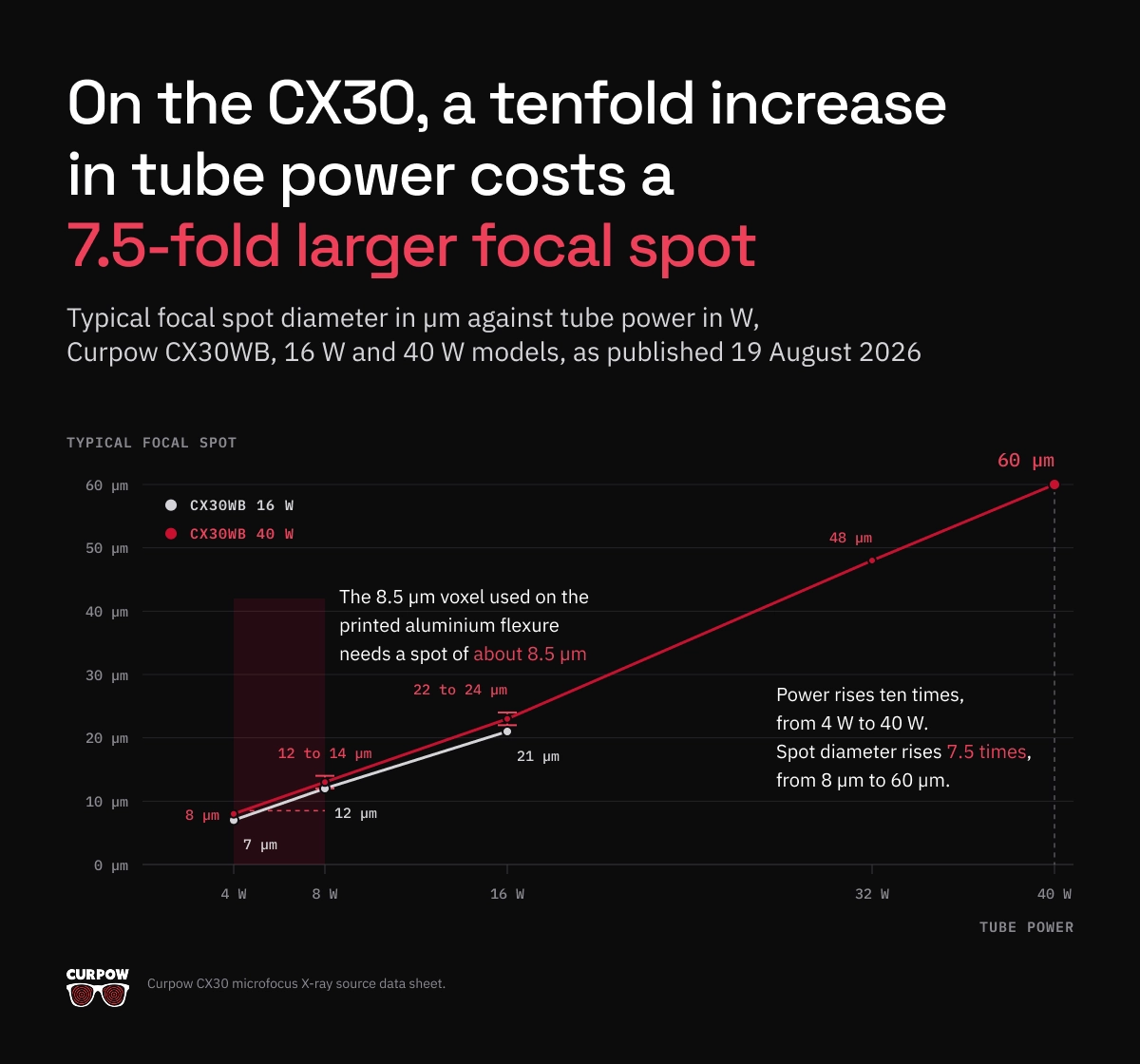
The CX30 curve tracks that 1 µm per watt rule closely. On the 16 W model, going from 4 W to 16 W adds 12 W and adds 14 µm of spot diameter. Read down the 40 W column and the trade is starker. Power rises ten times, from 4 W to 40 W. Spot diameter rises 7.5 times, from 8 µm to 60 µm. Because spot area follows the square of diameter, the area grows about 56 times, so power per unit area at the target falls to roughly 18 percent of its 4 W value.
Now map the CX30 curve onto the published scans. The 8.5 µm voxel used on the printed aluminium flexure needs a spot of about 8.5 µm, which the CX30 delivers between 4 W and 8 W. The 2.1 µm voxel on the ruby sphere standard needs a spot no source in the Curpow range reaches. That scan ran on a transmission target tube, where the electrons pass through a thin target rather than coming off a thick one, and that tube’s published JIMA resolution runs from 0.6 µm upward depending on the operating parameters.
When a CT system needs the smallest spot Curpow builds rather than the most flux, the CX40 reaches 4.5 µm on the wide-beam variant, and its data sheet names micro-CT and semiconductor inspection directly.
How to choose tube voltage for micro CT
Voltage follows the part. Published micro CT scans span a wide band, and the band maps onto material and path length rather than onto the application name.
At the low end, the team scanning the ruby sphere standard used 80 kV, because the beam crossed a few millimetres of ceramic. In the middle, a 30 mm by 12 mm by 5 mm aluminium printed part needed 145 kV. In semiconductor packaging, the Intel and Lawrence Livermore review reports that beams above 100 kV are usual, because copper and solder absorb heavily.
Raising kV costs you twice. The Intel and Lawrence Livermore review states that higher energy blooms the beam spot, so resolution falls away exactly where you needed the penetration. Higher energy also reduces phase contrast and makes the organic packaging materials invisible, so the same paper argues for brightness at lower energies rather than more kV.
So the specification question is whether a source gives you enough flux at the kV your material needs, rather than the highest kV it reaches. Across the range, the CX40 reaches 90 kV, the CX20 reaches 110 kV, and the 130 kV CX30 sits at the top.
Beam geometry belongs in the same decision. The CX30 puts out a 115 degree round beam with a uniform profile, which suits automated inspection and off-angle views. The CX40 offers 108 degrees on the wide beam and 40 degrees on the narrow beam, plus a side-window configuration at 34 degrees for compact enclosures. All three use a tungsten (W) target behind a beryllium (Be) window.
Spot position stability over a scan that runs for hours
Specify spot position stability next to spot size, because a stable 8 µm spot out-reconstructs an unstable 5 µm spot every time. The National Physical Laboratory and the Swiss federal metrology institute have both measured how far a focal spot moves during a scan, and what that movement costs a measurement.
The National Physical Laboratory, working with Nottingham and Southampton, ran 38 scans over three months on a 225 kV system at tube power below 6 W, with the reference object magnified about 130 times. After the tube ran for 20 minutes to reach thermal equilibrium, no scan showed spot drift above 0.15 µm across 10,000 seconds. A cold start behaved differently. The tube temperature climbed for the first eight minutes, and during those eight minutes the spot moved about 0.15 µm in one axis and 0.3 µm in the other. Across an eleven hour scan the spot moved 0.6 µm. Below 6 W the mechanical structure carrying the rotation stage drifted more than the focal spot did.
The Swiss federal metrology institute measured the same effect at the other end of the scale. Uncompensated thermal expansion of the tube head ran to about 10 µm along the magnification axis, on scans reconstructed at a 2.1 µm voxel. Correcting for the tube position cut the standard deviation on 231 sphere centre to centre distances from 0.20 µm to 0.11 µm. After a 15 minute warm-up, the compensated spot held within 0.5 µm parallel to the detector and 1 µm along the magnification axis. The same team requires its centring routine to land within a fraction of a voxel. For a 1 µm voxel that means 0.1 µm.
Three practical consequences follow, and none of them need new hardware:
- Warm the source up before the scan rather than starting cold.
- Expect the largest spot movement in the first ten minutes of X-ray production.
- Treat filament replacement as a recalibration event. The Swiss federal metrology institute logged tube position shifts of 8.4 µm to 24.1 µm after opening and closing the cathode chamber for maintenance.
Curpow states spot position stability on two data sheets. The CX30 sheet lists a highly stable spot position for CT and 3D imaging. The CX20 sheet lists high flux and spot location stability, for consistent imaging with minimal variation over time. Both sources also carry automatic source conditioning, which ramps the source up gradually after it has been off, and a digital RS-232 interface exposing diagnostics and operating logs. On a CT system those logs let you trace a reconstruction problem back to the source instead of to the stage.
Focus to object distance and the magnification your part leaves you
Your part decides how close it can get to the focal spot, and the source housing decides how close it may come. Together those two clearances fix your magnification, and no reconstruction software recovers detail the geometry never captured.
One NASA Jet Propulsion Laboratory study lost a measurement to exactly that clearance. The team put a four-high stacked package assembly through CT to find thermal cycling damage that optical microscopy had already seen. The board assembly stood slightly taller than the package itself, so the team could not bring the part in far enough, and the scan never reached maximum magnification. The reconstruction showed the stack geometry but never revealed the lead separation. On column grid array assemblies the same system resolved gross column tilt and nothing finer, and the study attributes the shortfall to lower magnification. The physics was fine. The clearance was not.
So a data sheet’s spot to window distance decides what your machine can resolve. The Swiss metrology institute reached 96 times magnification by placing its rotary axis 10.4 mm from the source, with the detector 997.4 mm away. Curpow’s three sources sit in that same band: the CX40 at 6.0 mm on the wide beam, the CX20 at 7.5 ± 1.0 mm, and the CX30 at 10 ± 0.5 mm from spot to window. The CX30 sheet credits that 10 mm spacing for the high geometric magnification it delivers, and the window is uncollimated at roughly 38 mm across on the wide beam.
Two numbers belong in your own design review:
- The closest approach your largest part allows, including its fixture and the swing it needs as it rotates.
- The spot to window distance of the source you are considering, so you can check the source does not spend that clearance before the part gets a share of it.
Choosing between the CX20, CX30, and CX40 for a micro CT system
Curpow designs all three sources low powered and high kV, which is the correct trade for CT work.
| CX20 | CX30 | CX40 | |
|---|---|---|---|
| Maximum tube voltage | 110 kV | 130 kV | 90 kV, 80 kV side-window |
| Minimum focal spot | 5 µm narrow beam, 7 µm wide beam | 7 µm at 4 W, see FIGURE 1 for the full curve | 4.5 µm wide beam, 5 µm narrow, 15 µm side-window |
| Maximum power | 25 W | 16 W or 40 W model | 8 W |
| Beam angle | 90° narrow, 125° wide | 115° round, uniform profile | 108° wide, 40° narrow, 34° side-window |
| Focus to object distance | 7.5 ± 1.0 mm | 10 ± 0.5 mm spot to window | 6.0 mm wide beam |
| Target and window | Tungsten (W) target, beryllium (Be) window | W target, Be window 0.51 mm | W target, Be window |
| Control interface | RS-232, digital | RS-232 digital, Windows GUI supplied | RS-232 digital on wide beam, analog available |
| Weight | 5.7 kg | 8.6 kg | 3.6 kg |
Specifications from the CX20, CX30, and CX40 data sheets, typical values.
Read the table as three positions on the same trade:
- The CX40 gives you the smallest focal spot in the range at 4.5 µm and the shortest approach at 6.0 mm, so it suits small dense parts scanned at the finest voxel your detector supports.
- The CX20 gives you the most flux in the range at 25 W and reaches 110 kV, which is what shortens a scan or feeds an automated inspection station.
- The CX30 gives you the highest voltage at 130 kV, the published focal spot against tube power curve, and the stability claim written for CT and 3D.
All three data sheets name micro-CT among their applications. Curpow’s own target list also names microfocus inspection of batteries, mini LEDs, and printed circuit boards. Read the board and package side of that work on the PCB and electronics inspection page, and the cell side on the battery cell inspection page.
Lead time and second sourcing
Curpow designs and manufactures microfocus X-ray sources, high voltage low power X-ray modules for integrated sources, and stand-alone X-ray power supplies. Those parts go inside the CT systems that inspection OEMs and integrators build. Curpow also builds application-specific turnkey inspection systems.
Lead time is six weeks. For a CT system builder that number lands in two places. Lead time sets how fast you can bring a new machine configuration to a customer trial, and it sets how long a fielded scanner sits idle when a source fails. Buyers fund second-source qualification because of the idle scanner, not because of the customer trial.
Curpow started in 2022 in Santa Cruz, California, and carries the 50 year Kevex legacy in focused X-rays. Curpow holds an ISO 9001 certification from an ANAB accredited certification body. In 2025 Thermo Fisher Scientific named Curpow a preferred contract manufacturing partner.
How to specify an X-ray source for your CT system
- Name the smallest feature the scan has to resolve, with a dimension. You can specify against “a 30 µm pore in a 5 mm aluminium wall”. You cannot specify against “high resolution”.
- Work the voxel back from that feature, then set the spot equal to it. A feature only a few voxels across is already the hard case, as the printed flexure study found at 30 µm holes on an 8.5 µm voxel.
- Fix the power your exposure budget needs before you read any spot figure. Projection count multiplied by exposure per projection is your scan time, and your customer is buying scan time.
- Ask for focal spot against tube power as a curve, not a minimum. A minimum spot and a maximum power on the same sheet describe two operating points that never coincide. If nobody will give you the curve, you do not yet know what the source does in your duty cycle.
- Set kV from the material and the path length, not from the application. Then ask for flux at that kV rather than for a higher ceiling you will never use.
- Specify spot position stability separately from spot size, and state the scan duration it has to hold across. Ask about warm-up behaviour too, because a cold start moves the spot most in the first ten minutes.
- Measure the clearance your largest part needs, fixture and rotation included, and check the source’s spot to window distance against it. Spot to window distance is the specification the JPL study came unstuck on.
What this means for your source selection
Geometry decides most of what a micro CT system can do, and software decides little of it. The voxel comes from the magnification. The magnification comes from how close the part can sit to the focal spot. The useful resolution comes from how large that focal spot is and how still it holds while the turntable works its way round. Every one of those is a source specification, so the source is the component to settle first, and the one your customers will judge the finished scanner on.
If you are specifying a source for a CT system now, send us the smallest feature you have to resolve, the material and thickness the beam has to cross, and your scan time budget. We will tell you which of the three fits and at what operating point. Talk to Curpow engineering. Browse our other applications on the applications hub.
Sources
“Investigation of the Focal Spot Drift in Industrial Cone-beam X-ray Computed Tomography”. Nadia Flay, Wenjuan Sun, and Stephen Brown, Engineering Measurement Division, National Physical Laboratory, with Richard Leach, University of Nottingham, and Thomas Blumensath, University of Southampton; Digital Industrial Radiology and Computed Tomography (DIR 2015), Ghent, June 2015; conference paper, full text. Thirty-eight scans over three months on one 225 kV cone beam system, tube power held below 6 W, reference sphere magnified about 130 times.
“X-ray source tracking to compensate focal spot drifts for dimensional CT measurements”. Benjamin A. Bircher, Felix Meli, Alain Küng, and Rudolf Thalmann, Laboratory for Length, Nano- and Microtechnology, Federal Institute of Metrology METAS, Bern; 10th Conference on Industrial Computed Tomography (iCT 2020), Wels; conference paper, full text. A 22-sphere ruby standard of 3.6 mm overall length, scanned at 80 kV and 5 W at 96 times magnification. The scan ran 3,000 projections over 5 hours and reconstructed at a 2.1 µm voxel, and the authors compared the result against a tactile measurement calibrated to 0.08 µm.
“Review of high-speed imaging with lab-based x-ray computed tomography”. E. A. Zwanenburg, M. A. Williams, and J. M. Warnett, WMG, University of Warwick; *Measurement Science and Technology* 33(1):012003, 19 November 2021; peer-reviewed review, open access, full text. A survey of published fast and in-situ laboratory CT work, reporting acquisition times, projection counts against the Nyquist criterion, and the power, spot size, and binning trade-offs operators use to reach them.
“High Resolution and Fast Throughput-time X-ray Computed Tomography for Semiconductor Packaging Applications”. Yan Li, Mario Pacheco, and Deepak Goyal, Assembly Test and Technology Development Failure Analysis Labs, Intel Corporation, with John W. Elmer and Holly D. Barth, Materials Engineering Division, Lawrence Livermore National Laboratory, and Dula Parkinson, Advanced Light Source, Lawrence Berkeley National Laboratory; IEEE Electronics Components and Technology Conference, 2014, LLNL-PROC-651694; conference paper, full text. A review of laboratory CT applied to microelectronic packages, alongside synchrotron scans of a 16 mm by 16 mm system in package at 4.5 to 8.7 µm resolution in 3 to 20 minutes.
“Development of a modular system to provide confidence in porosity analysis of additively manufactured components using x-ray computed tomography”. Y. Chahid, C. Packer, A. Tawfik, J. Keen, N. Brewster, M. Beardsley, K. Morris, P. Bills, L. Blunt, C. Atkins, and S. Tammas-Williams, STFC UK Astronomy Technology Centre, with the University of Edinburgh, the University of Huddersfield, RALSpace, and the University of Lincoln; *Measurement Science and Technology* 35(4), 2024; peer-reviewed study, open access, full text. An additively manufactured aluminium flexure hinge of 30 mm by 12 mm by 5 mm scanned at 145 kV and 41 µA over 1,650 projections at an 8.5 µm voxel, against a micro-machined reference pin with calibrated 30, 50, 90, and 120 µm internal holes.
“Ghaffarian, R. 3D X-ray CT for BGA/CGA Workmanship Defect Detection. JPL Publication 12-21, NASA NEPP, December 2012″. Reza Ghaffarian, Jet Propulsion Laboratory, California Institute of Technology, for the NASA Electronic Parts and Packaging Program; 2012; agency technical report, full text. Column grid array assemblies and a four-high stacked thin small outline package assembly inspected by 2D radiography and CT after thermal cycling, on a system rated to 2,800 times geometric magnification.
“Voxel Size Calibration for High-resolution CT”. Marek Zemek, Pavel Blažek, Jakub Šalplachta, Tomáš Zikmund, and Jozef Kaiser, Central European Institute of Technology, Brno University of Technology, with Jan Šrámek and Petr Klapetek, Czech Metrology Institute, and Yoshihiro Takeda and Kazuhiko Omote, Rigaku Corporation; 10th Conference on Industrial Computed Tomography (iCT 2020), Wels; conference paper, full text. A calibration method for high-resolution systems with a field of view around one millimetre, stating voxel size as detector pixel pitch divided by cone beam magnification.
“An overview of industrial X-ray computed tomography”. Wenjuan Sun, Stephen B. Brown, and Richard K. Leach, National Physical Laboratory; NPL Report ENG 32, January 2012; national metrology institute report, full text. A survey of industrial CT covering source and detector technology, the focal spot size bands that define conventional, microfocus, and nanofocus systems, artefact definitions from ISO 15708, and the results of an international comparison audit of reference artefacts across fifteen CT systems.
“CX30 Microfocus X-Ray Source”, “CX20 Microfocus X-Ray Source”, and “CX40 Microfocus X-Ray Source” data sheets, plus the Curpow company page. Curpow Inc.; manufacturer specifications, typical values; CX30 sheet dated 19 August 2026.
FAQ
Direct answers
Frequently asked questions about X Ray sources for Micro CT and Industrial CT Systems
What focal spot size does a micro CT system need?
Match the focal spot to the voxel size the reconstruction uses. Published practice in laboratory CT is to set tube power at the point where spot diameter is similar to voxel size, because a smaller spot only costs exposure time and a larger spot wastes the detector sampling. A system reconstructing at a 5 µm voxel therefore needs a source holding about a 5 µm spot at the power that scan runs at. Microfocus sources cover 1 µm to 1000 µm of focal spot, and nanofocus sources go below 1 µm.
Why does focal spot size change with tube power?
About 1 percent of the energy an X-ray tube consumes leaves as X-rays and the remaining 99 percent becomes heat in the target. The focal spot is the area where the electron beam lands, and the target tolerates a limited amount of power per unit area, so extra power has to spread over extra area. A published review of high-speed laboratory CT gives the working rule for most X-ray sources: spot diameter grows about 1 µm per watt. Curpow’s CX30 data sheet gives the measured curve: a typical focal spot of 7 µm at 4 W, 12 µm at 8 W, and 21 µm at 16 W on the 16 W model, reaching 60 µm at 40 W on the 40 W model.
What tube voltage does micro CT need?
Voltage depends on the material and the path length the beam crosses, not on the word micro CT. Published scans ran 80 kV through a few millimetres of ruby and ceramic, 145 kV through a 30 mm by 12 mm by 5 mm aluminium printed part, and above 100 kV on copper and solder inside semiconductor packages. Higher voltage costs resolution, because the beam spot blooms at higher energy, and it also flattens the contrast that makes organic packaging materials visible. Curpow’s range spans 90 kV on the CX40, 110 kV on the CX20, and 130 kV on the CX30.
How much can the focal spot drift before it spoils a CT reconstruction?
Keep drift to a fraction of the voxel size the scan reconstructs at. The Swiss federal metrology institute targets 0.1 µm of centring accuracy for a 1 µm voxel, and measured about 10 µm of uncompensated tube thermal expansion on scans reconstructed at a 2.1 µm voxel, which is roughly five voxels of movement. Correcting for the expansion cut the standard deviation on 231 calibrated sphere centre to centre distances from 0.20 µm to 0.11 µm. Separately, the National Physical Laboratory found that a tube held below 6 W and warmed up for 20 minutes kept spot drift under 0.15 µm across 10,000 seconds of scanning.
What is the difference between micro CT and conventional CT?
Focal spot size separates them. Conventional CT systems run focal spots larger than 1 mm, microfocus systems run 1 µm to 1000 µm, and nanofocus systems go below 1 µm. Because the spot casts the blur that limits resolution, a millimetre-scale spot cannot resolve micrometre-scale detail at any magnification. Industrial micro CT also rotates the part in front of a fixed source and detector. So the part has to fit between the two and clear the source housing as it turns. That is what limits the magnification available on a large assembly.
Can micro CT run in line on a production line?
Yes, and an in-line scan pays for the speed with projections and focal spot size. A dimensional laboratory scan of a 3.6 mm sphere standard at a 2.1 µm voxel took 3,000 projections and five hours, and a published survey puts the fastest commercial scan at 9.4 seconds. That survey also found that operators chasing speed run about 60 percent of the projections the Nyquist criterion asks for, and that two by two detector binning brightens the image four times so exposure per projection falls proportionally. An in-line CT station therefore needs flux above all, while a laboratory system needs the smallest stable spot.
Which Curpow source suits a micro CT system?
All three name micro-CT on their data sheets, and they sit at different points on the same trade. The CX40 holds the smallest focal spot at 4.5 µm on the wide beam and the shortest focus to object distance at 6.0 mm, for small dense parts at fine voxels. The CX20 carries the most power at 25 W and reaches 110 kV, which shortens scan times and suits automated stations. The CX30 reaches 130 kV, publishes its full focal spot against tube power curve, and lists a highly stable spot position for CT and 3D imaging. Lead time is six weeks on all three.